Why I Chose TimescaleDB Over ClickHouse for Analytics (Part 1)
When you build a web analytics product that tracks page views, sessions and web performance metrics, the database sits at the core of both the product and the architecture. When I started building witnes.io, the first version ran on plain PostgreSQL tables, with a lot of heavy queries that concatenated and grouped data across raw and aggregated tables.
That was fine for a proof of concept. It was also obvious it would not scale well.
When I re-architected the data layer, the choice came down to two options: TimescaleDB or ClickHouse.
ClickHouse seems to be the default answer these days for high-volume analytics, and I still went with TimescaleDB. What tipped the scale was operational sanity and familiarity, combined with a realistic look at the numbers: witnes would not be processing more than a few hundred million data points.
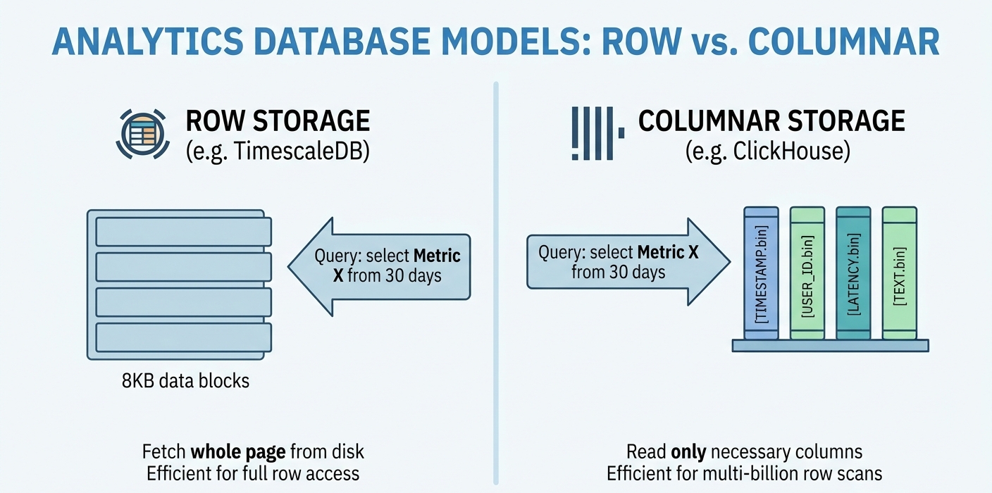
1. Row vs. columnar
The two databases have the same aim, but they store (and therefore process) data in opposite ways.
Row storage (PostgreSQL / TimescaleDB)
PostgreSQL stores data row by row. Each entity gets one row, split into columns, much like an Excel sheet.
Now ask a question like “what was the average latency over the last 30 days?“. A row database has to read the whole row off the disk and move it into RAM (TOAST aside), pulling in IDs and other fields you never asked for, just to compute one number. That is true even if you only selected that one column.
Columnar storage (ClickHouse)
ClickHouse takes a 90 degree turn. Every column of a table is stored in its own file on disk. ColumnA becomes columnA.bin.
Ask the same question again and the query is dramatically faster, because the database only has to open columnA.bin and can ignore every other field on disk.
This makes the columnar approach an absolute beast at scanning billions of rows across a single attribute. The catch is that it is an entirely different database paradigm, with its own nuances and its own infrastructure footprint.
How TimescaleDB competes
So how does TimescaleDB compete with that? By having a clearly defined scope. witnes, for example, does not need any aggregation finer than one day. When you know that, you can tune TimescaleDB very finely, using a few of its tools:
- Hypertables. A hypertable looks like a normal table, but underneath it slices the data into smaller tables called chunks, built from time intervals (this is where the defined scope helps). When a query asks for a specific date range, partition pruning skips every irrelevant chunk, so the database looks at far less data.
- Compression. This feels a bit like cheating: older chunks can be compressed into a columnar format under the hood. You have to pick carefully which columns you filter by, and it works best for “cold” data. In witnes, data is considered cold after 30 days. Recent data stays fast to write, and older data falls back to the compressed form. Again, a well-defined scope is what lets you tune this.
- Continuous aggregates. Everyone who uses PostgreSQL knows materialized views, and everyone wished they were better. TimescaleDB lets you keep real-time materialized views that refresh incrementally in the background.
TimescaleDB has many more features that speed up your data. I will cover some of them in Part 2.
2. Operational simplicity and PostgreSQL familiarity
If we use every trick available, ClickHouse still wins on raw performance at petabyte scale. But performance is not the only thing that matters in a product and in engineering. TimescaleDB won because of how simple it is to set up, run, and develop against.
It is an extension. It runs on top of the database you already have. Running ClickHouse in production means introducing a new database architecture that you have to learn and maintain, even if you use a hosted solution. TimescaleDB can be adopted inside your existing PostgreSQL.
It is opt-in. Every feature is optional. Your system can keep using standard PostgreSQL tables and queries with your everyday ORMs, and you opt into the advanced features only when you need them.
3. How witnes.io is structured around TimescaleDB
In witnes, TimescaleDB is the base of a multi-layered pipeline built on the Medallion Architecture.
Raw ingestion hypertables (bronze, silver, gold). They are chunked in 1-day intervals. Data is kept uncompressed while it is hot. After 30 days it is segment-compressed, using tenant and project as the segmenting columns. There is also a hard physical retention window of one year: anything older is dropped.
Continuous aggregates. Six materialized views replace the multiple tables that used to be maintained by background jobs.
Ingestion never stops. The ingestion of data never stops for any user regardless of their pricing tier. The setup leaves a lot of headroom for processing, so if a user upgrades later, the data they would want is already there.
Summary
For a bigger product, I would seriously consider ClickHouse, for the peace of mind that performance problems would show up later rather than sooner. But engineering resources are slim, and TimescaleDB gave me the best of both worlds: it handles big amounts of data, with a low barrier to entry.
Ready to dive into the math? In Part 2, we will look at how I solved the age-old problem of multi-day distinct counts and percentiles, using HyperLogLog (HLL) and t-digest sketches inside continuous aggregates.